Bias Adjustment
All estimated gridded data (satellite rainfall estimates, models output, …) are subject to different types of errors, including errors from sensors, algorithms and random errors.
There are two main sources errors for the estimated gridded data: random error and systematic bias. These discrepancies between the estimated gridded data and the station observations need to be corrected before further analysis. The systematic bias can be reduced or eliminated by applying statistical bias correction methods.
Computing Bias coefficients
CDT uses an approach based on historical data from the estimated gridded data and station observations to correct the systematic bias. A climatological bais coefficients are first computed for each month or at the temporal resolution of the data.
The color light blue of the menu means that you only need to compute the bias coefficients once. Indeed, you will need a long series and quality controlled station data to compute the climatological bias coefficients. Once the coefficients are calculated you can use it to correct the systematic bias from the same source of the estimated gridded data.
Climate data
The menu allows to compute the climatological bias coefficients for rainfall, temperature, relative humidity, radiation and pressure data.
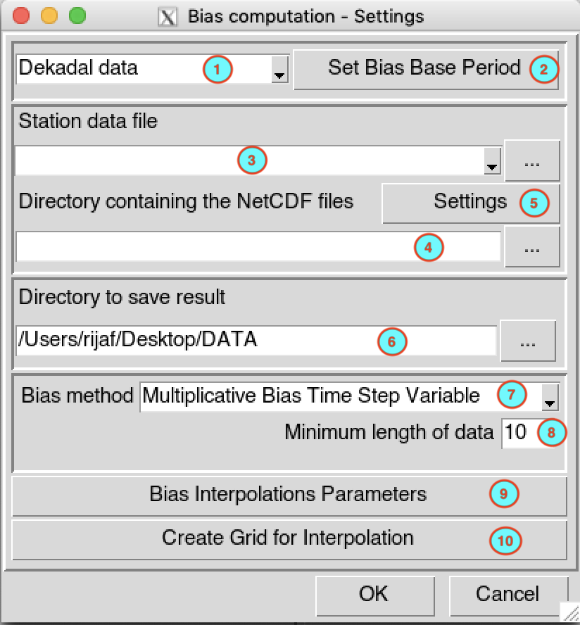
Select the temporal resolution of the data. Available temporal resolution are: daily, pentad, dekadal and monthly data.
Click on the button to specify the period and minimum number of year to be use to compute the bias coefficients. All the parameters can be set in the base period setting dialog.
Select the file containing the station data (in CDT station data format) to use from the drop down list if it is already loaded, or open it through
 .
.Type the full path to the folder containing the netCDF files or browse it from the button
on the
right.Provide a netCDF sample file and change the filename format of the netCDF file through the netCDF settings dialog by clicking on the button .
Type the full path to the folder to save the computed bias coefficients, or use the browse button
.Select the method to use to compute the bias coefficients. CDT has 4 methods to compute the bias coefficients: Multiplicative Bias Time Step Variable, Multiplicative Bias for Each Month, Quantile Mapping with Fitted Distribution, and Quantile Mapping with Empirical Distribution. See CDT bias adjustment methods section for more information.
Enter the minimum length of non missing values to be used to calculate the bias coefficients or to fit the distribution. Although you already specify the minimum number of year needed to compute the bias coefficients, it is possible that some dekads and months contain missing values, you need to specify here the minimum length of data to be used to perform the computation.
Click on the button to open the interpolation dialog to select the interpolation method to be used and set the all parameters for the interpolation.
Click on the button to create the grid to be used to interpolate the data. It will display the grid creation dialog box.
Click on the button  to run
the bias coefficients calculation.
to run
the bias coefficients calculation.
A folder named BIAS_Data_<file name of station data> will be created under the folder you provided (6) to save the outputs. This folder contains a file named BIAS_PARAMS.rds containing the parameters used to computed the bias coefficients, and one or more files depending on the method used.
- Multiplicative Bias Time Step Variable: a netCDF files named STN_GRD_Bias_Coeff_<n>.nc, where \(n\) is the \(n^{th}\) bias coefficients. The total number of bias coefficients \(N\) is
\[ N = \begin{cases} 365, & \text{ for daily data} \\ 72, & \text{ for pentadal data} \\ 36, & \text{ for dekadal data} \\ 12, & \text{ for monthly data} \end{cases} \]
- Multiplicative Bias for Each Month: a netCDF files named STN_GRD_Bias_Coeff_<n>.nc, where \(n\) is the bias coefficient of the \(n^{th}\) month.
- Quantile Mapping with Fitted Distribution: a netCDF files named STN_Bias_Pars_<distname>_<n>.nc containing the computed and interpolated distribution parameters for stations data and GRD_Bias_Pars_<distname>_<n>.nc for the gridded data; where distname is the fitted distribution name BernGamma for rainfall and Gaussian for the other variables; \(n\) is the bias coefficient of the \(n^{th}\) month.
- Quantile Mapping with Empirical Distribution: a file named GRID_DATA.rds containing the quantile functions of the empirical distribution.
Wind data
The menu allows to compute the climatological bias coefficients for wind data.
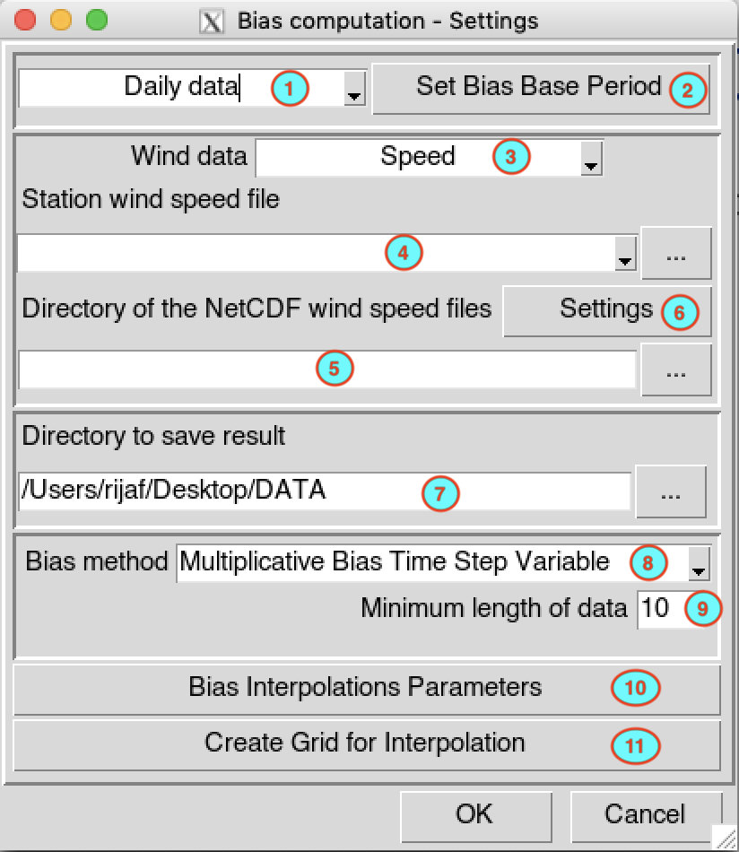
Select the temporal resolution of the data. Available temporal resolution are: daily, pentad, dekadal and monthly data.
Click on the button to specify the period and minimum number of year to be use to compute the bias coefficients. All the parameters can be set in the base period setting dialog.
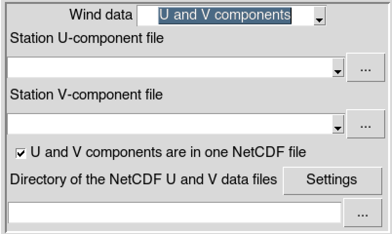
Select the wind variables to be used: wind speed only or the U and V components of the wind data.
If the wind speed is selected in (3), provide the file containing the wind speed data (in CDT station data format) to use. In case of U and V components, you have to provide the files containing the station data for U-component and V-component of the wind data. You can select the files from the drop down list if it is already loaded, or open it through
.
- If the wind speed is selected in
(3), type the full path to the folder containing the
netCDF files or browse it from the button on the right. In case of
U and V components, provide the full path to
the folder containing the netCDF wind data files; if the U and V
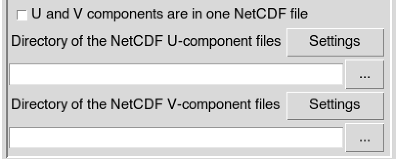
components are stored in separate files, uncheck
 U and V components are in one NetCDF file
and provide the full paths to the folder containing the
netCDF U-component and V-component files.
U and V components are in one NetCDF file
and provide the full paths to the folder containing the
netCDF U-component and V-component files.
Provide a netCDF sample file and change the filename format of the netCDF file through the netCDF settings dialog by clicking on the button .
Type the full path to the folder to save the computed bias coefficients, or use the browse button
.Select the method to use to compute the bias coefficients. CDT has 4 methods to compute the bias coefficients: Multiplicative Bias Time Step Variable, Multiplicative Bias for Each Month, Quantile Mapping with Fitted Distribution, and Quantile Mapping with Empirical Distribution. See CDT bias adjustment methods section for more information.
Enter the minimum length of non missing values to be used to calculate the bias coefficients or to fit the distribution. Although you already specify the minimum number of year needed to compute the bias coefficients, it is possible that some dekads and months contain missing values, you need to specify here the minimum length of data to be used to perform the computation.
Click on the button to open the interpolation dialog to select the interpolation method to be used and set the all parameters for the interpolation.
Click on the button to create the grid to be used to interpolate the data. It will display the grid creation dialog box.
Click on the button to
start the bias coefficients calculation.
A folder named BIAS_Wind_Data will be created under the folder you provided (7) to save the outputs. This folder contains a file named BIAS_PARAMS.rds containing the parameters used to computed the bias coefficients, and one or more files depending on the method used. The names of the created files are the same as the output of the bias coefficients for the climate data.
Apply bias correction
Climate data
The menu allows to adjust the systematic bias of the gridded data (rainfall, temperature, relative humidity, radiation and pressure variables).
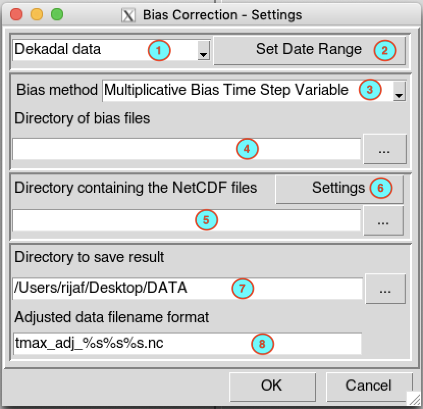
Select the temporal resolution of the data. Available temporal resolution are: daily, pentad, dekadal and monthly data.
Set the start and end date of the period over which the bias of the gridded data will be adjusted. See setting date range for more details.
Select the method to use to compute the bias coefficients. CDT has 4 methods to compute the bias coefficients: Multiplicative Bias Time Step Variable, Multiplicative Bias for Each Month, Quantile Mapping with Fitted Distribution, and Quantile Mapping with Empirical Distribution. See CDT bias adjustment methods page for more information.
Provide the full path to the folder containing the bias coefficients.
Type the full path to the folder containing the netCDF files or browse it from the button
on the
right.Provide a netCDF sample file and change the filename format of the netCDF file through the netCDF settings dialog by clicking on the button .
Type the full path to the folder to save the bias adjusted data, or use the browse button
.Specify the netCDF filename format of the output files.
Click on the button to
start the bias correction.
A folder named ADJUSTED_<name of climate variable>_Data_<start date>_<end date> will be created under the folder you provided (7) to save the outputs. It contains the bias corrected climate data in netCDF format.
Wind data
The menu allows to adjust the systematic bias of the gridded wind data.
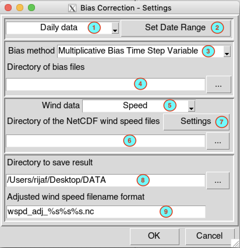
Select the temporal resolution of the data. Available temporal resolution are: daily, pentad, dekadal and monthly data.
Set the start and end date of the period over which the bias of the gridded data will be adjusted. See setting date range for more details.
Select the method used to compute the bias coefficients. CDT has 4 methods to compute the bias coefficients: Multiplicative Bias Time Step Variable, Multiplicative Bias for Each Month, Quantile Mapping with Fitted Distribution, and Quantile Mapping with Empirical Distribution. See CDT bias adjustment methods section for more information.
Provide the full path to the folder containing the bias coefficients.
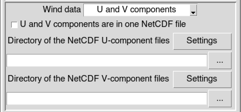
Select the wind variables to be adjusted: wind speed only or the U and V components of the wind data.
If the wind speed is selected in (5), type the full path to the folder containing the netCDF files or browse it from the button
on the right. In case of
U and V components, provide the full path to
the folder containing the netCDF wind data files; if the U and V
components are stored in separate files, uncheck
U and V components are in one NetCDF file
and provide the full paths to the folder containing the
U-component and V-component netCDF files.
Provide a netCDF sample file and change the filename format of the netCDF file through the netCDF settings dialog by clicking on the button .
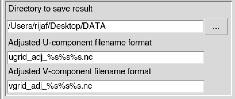
Type the full path to the folder to save the bias adjusted wind data, or use the browse button
.Specify the netCDF filename format of the output files. In case of U and V components stored in different files, specify the netCDF filename format for each component.
Click on the button to
start the bias correction.
A folder named ADJUSTED_Wind_Data__<start date>_<end date> will be created under the folder you provided (8) to save the outputs. It contains the bias corrected wind data in netCDF format.