Subseasonal forecasting set-up
Forecast issuing schedule
Subseasonal forecasts are typically issued once a week, though this varies between forecasting centers, especially for the S2S database models; see this S2S table. For example, ECMWF issues forecasts twice a week, every Monday and Thursday. The forecasts extend 4–8 weeks into the future, with the model output provided every day. However, subsesaonal forecasts are typically expressed as weekly or biweekly time averages.
A simple set up:
Week 1: Lead days 1-7
Week 2: Lead days 8-14
Week 3: Lead days 15-21
Week 4: Lead days 22-28
and:
Weeks 2–3: Lead days 8-21
Weeks 3–4: Lead days 15-28
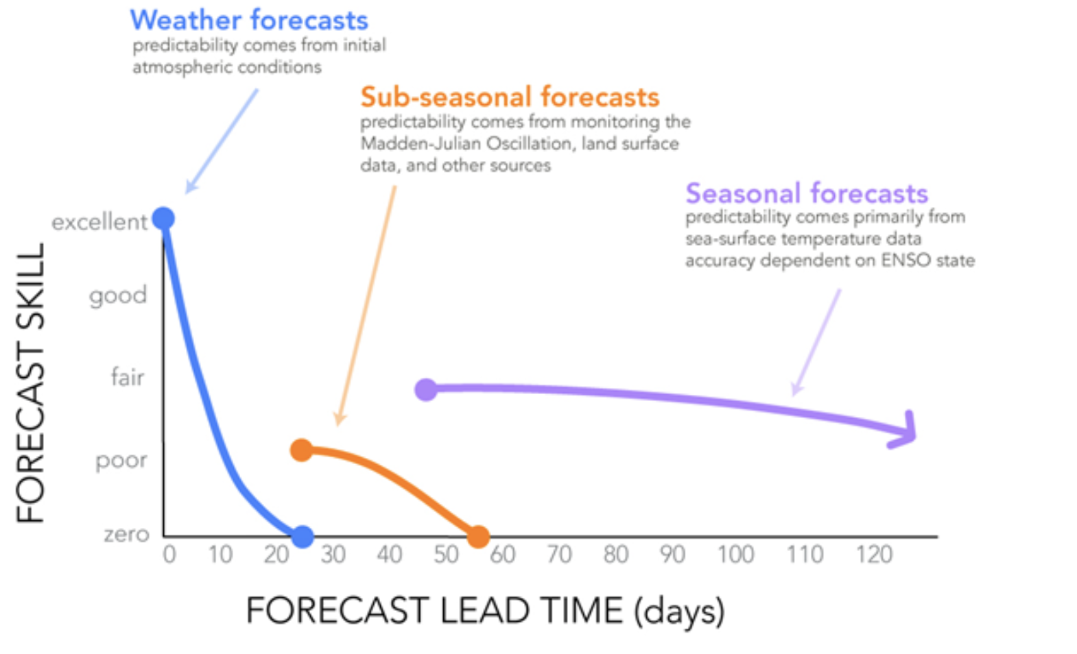
Time averaging increases the predictability by increasing the S/N ratio (e.g., averaging out daily weather noise), with a trade-off against less temporal specificity. Weeks 3–4 is a “sweet spot”: higher predictability from averaging over 2 weeks, while the two-week window is often precise enough for societal decisions 3–4 weeks ahead.
The above daily lead-time ranges are often shifted slightly in operational forecast products because it takes a few days for the model’s forecast data to become available, for the post-processing to be run, and for the forecast to be issued on a website. For example, IRI’s Subseasonal forecasts issued every Friday* use SubX model forecasts made (initialized) on Wednesday, for target weeks starting on Saturday. Here Week 1 is defined as Days 4-10, and so on; the ranges above would thus need to be incremented by +3.
The SubX forecasts are mostly initialized on Wednesdays. The S2S project forecasts are all initialized on Thursdays, but there is a 3-week embargo in their availability for operational reasons.
Hindcasts
Like seasonal forecasts, subseasonal forecasts contain biases (e.g., too wet/too dry) that can be corrected by using the results of hindcasts (aka “reforecasts”) where the forecasts are re-run for a large set of dates in the past. Because the S2S project forecasts are made by operational centers (Global Producing Centers in WMO parlance), their hindcast set-ups vary from center to center. The SubX project specified a hindcast protocol with hindcasts every week 1999–2016, making them easier to use.
PyCPT uses the hindcasts to bias-correct the forecasts by calibrating them against regional observed datasets using regression. This is more complex than in the seasonal forecasting case because of need for daily calendars and the diversity of forecast and hindcast set-ups.