Hidden Markov Models for Modeling of Daily Station Rainfall
![]()
![]()
![]()
Introduction
The Hidden
Markov Model (HMM) provides a framework for modeling daily rainfall occurrences
and amounts on multi-site rainfall networks. The HMM fits a model to observed
rainfall records by introducing a small number of discrete rainfallstates.
These states allow a diagnostic interpretation of observed rainfall variability
in terms of a few rainfall patterns. They are not directly observable,
or 'hidden' from the observer.
The time sequence
of which state is active on each day follows a Markov chain. Thus, the
state which is active 'today' depends only on the state which was active
'yesterday' according to transition probabilities.
The HMM also
allows you to simulate
rainfall at each of the station locations, such that key statistical properties
(eg. rainfall probabilities, dry/wet spell lengths) of the simulated rainfall
match those of the observed rainfall records. This can be useful for generating
large numbers of synthetic realizations of rainfall for input into statistical
analysis, or input into a crop simulation model, for example.
The HMM also
provides a basis for downscaling GCM simulations to the station scale,
or calibrating estimates of observed rainfall. Downscaling is accomplished
using a nonhomogeneous
HMM (NHMM) in which predictors are incorporated into the HMM. The predictors
modulate the transitions between the states over time. The transition
matrix is no longer homogeneous in time, hence the name.
The HMM toolbox
contains models of varying complexity that you can use to analyze sets
of rainfall observations. The HMM represents the rainfall-gauge observations
themselves, without any of the treatment needed to average the point-scale
observations onto grids. It represents the raw observations. Missing observations
are allowed, and a treated in a consistent probabilistic manner. Several
options are available for modeling spatial dependencies between stations.
The HMM can be
thought of as a cluster analysis of multi-site rainfall observations,
with an explicit (Markov chain) time dependence. In its ability to make
simulations, it also bears similarities to existing stochastic weather
generators.
This tutorial provides
a basic introduction to the use of the Toolbox for analysis of rainfall
observations, covering the capabilities in the GUI implementation.
Typical Usage of HMMTool
Launch HMMTool,
either from the command line (linux and Mac), or by double-clicking the
HMMTool icon (Windows). Please see the platform-specific installation
instructions for
each platform (Linux, Mac or Windows XP). This will bring up the Main
Frame of the HMMTool graphical user interface.
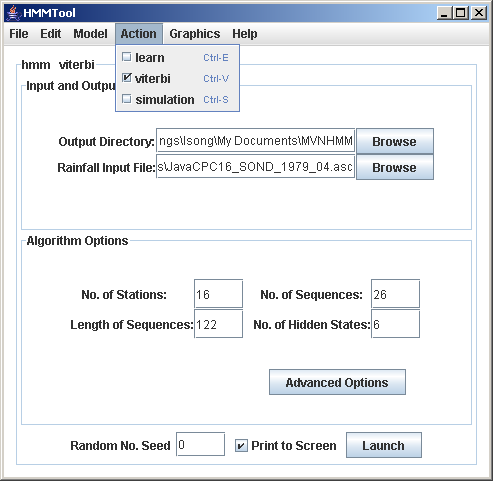
For a chosen model, analysis with HMMTool consists of a sequence of Actions, performed consecutively from the Action Menu at the top of the main frame. First estimate the model parameters (learn action), secondly estimate the most-likely state sequence (viterbi action), and thirdly generate rainfall simulations.
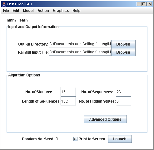
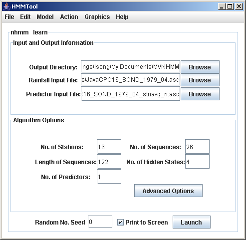
1.Describe Your Data
Using the Main Frame of HMMTool, select your rainfall data file, an output directory for the results files, and fill in the boxes specifying the number of stations, number of sequences (e.g. one for each summer season), length of sequences (i.e. number of days in each season), and number of hidden states. A 4-state model often makes a reasonable starting point. We return to the number of hidden states later. Apart from the number of states, which can be any value, the values specifying the size of the rainfall data set need to match your input file.At least two input files are needed: one containing the rainfall data, and one containing the longitude-latitude coordinates of the station. In the case for NHMM or NMIXTURE, an additional input file is needed for the predictors. In the rainfall data file, columns should correspond to stations, and rows to days.2.Choose the Model
Having filled in the basic options, the next step is to choose the model type from the Model Menu, and specify its details.a. Model Types There are 4 model types under the Model menu:
HMM - Hidden Markov ModelModel with first-order Markovian time dependenceNHMM - Nonhomogeneous Hidden Markov ModelHMM with predictors, sometimes called 'inputs.' These inputs consist of one or more daily real-valued timeseries. A logistic regression is used to model model the dependence of state-probability on the inputs.MIXTURE - Mixture modelModel without explicit time dependence. This is the same as the HMM, but without the modeled Markov time dependence.NMIXTURE - Nonhomogeneous Mixture modelModel MIXTURE with predictors.b. Specifying the Model Details
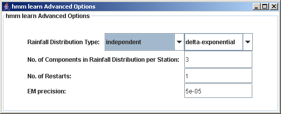
The way you wish to model the rainfall data is controlled under the Advanced Options tab, by specifying the spatial model and the rainfall distribution.Spatial ModelChoice of spatial model can be important to the properties of simulated rainfall in applications where capturing spatial correlations between stations may be important (e.g. hydrology). Two spatial models are available: (a) Independent, in which rainfall at each station is assumed independent of the other stations, or (b) Chow-Liu, in which spatial dependence is modeled using tree models.Please note that the Chow-Liu option is currently only working for certain choices of model. The Independent model is selected by default, and is sufficient in most cases. Some spatial dependence will be captured through the state variable even under the Independent model, for example if a state is characterized by high rainfall probabilities at all stations.Rainfall Distribution TypeHMMTool can model binary rainfall occurrence data, or real valued rainfall amounts. If the data are binary, then the Bernoulli distribution should be used. If the data are real, the rainfall amounts are modeled using a mixture of distributions, consisting of a delta-function at zero and a set of exponentials or gamma distributions. These two possibilities are named delta-exponential and delta-gamma respectively on the right of the Advanced Options panel. The number of components included in the mixture (including the delta function) needs to be entered in the line below. For example, the common (default) choice of a delta function together with two exponentials would be delta-exponential with 3 components entered. A delta function together with one gamma distribution would be delta-gamma with 2 components.Other Advanced OptionsThere are two further options for the learn action: Number of restarts, and EM precision. The number of restarts specifies how many times the EM algorithm is executed from different random starting points. HMMTool uses an iterative maximum likelihood method, selecting the restart with the highest log-likelihood as its best estimate of the global maximum in the likelihood. While larger numbers of restarts are preferable, this slows execution. Inspection of log-likelihood values in the output can help decide on an appropriate number. Typically, 10 is a relatively safe choice, but a much smaller number can be used for test purposes. The EM precision controls the stopping point of iteration, and can be left at its default value.3.Make a Preliminary Analysis
We are now ready to make our first analysis, performing the three actions consecutively from the Action Menu: estimate the model parameters (learn), estimate the most-likely state sequence (viterbi), and thirdly generate rainfall simulations (simulate).a. Learn Action
Make sure the learn is selected from the Action Menu. Select Launch from the main frame. Print to Screen prints the log-likelihood values at each iteration, although execution will have to be completed before anything appears. Random number seed allows for different starting points of the pseudo random number generator; the results are repeatable from each seed value.Execution times may be several minutes, and much longer on slower machines for large datasets with large numbers of hidden states.Once execution is complete, the results can be plotted from the Graphics Menu, as maps of rainfall probability and mean rainfall amount on wet days at each station. The mean rainfall amount (for delta-exponential and delta-gamma) is computed from the parametric form of the distribution.All the estimated model parameters are written to a *.out file in the specified output directory. The output filenames are based on the rainfall input filename, and include the action (here learn), model-type and options.b. Viterbi Action
Once the model parameters have been estimated, we are ready to estimate the most-likely state sequence, using the Viterbi action from the Action Menu. No options or advanced options need to be changed. Once Viterbi has been selected, simply click Launch on the Main Frame.Execution of the Viterbi action is rapid. Once it completes, a visualization of the state sequence can be viewed from the Graphics Menu. The sequence is written to a *.out file in the output directory, with a filename including the word 'viterbi.' Note that the states are numbered from 0 in this file, with 0 corresponding to state 1. Each row of the file contains a single temporal sequence, ordered from first to last.The Viterbi sequence can be used off-line to construct composites of atmospheric circulation, from reanalysis data.c. Simulate Action
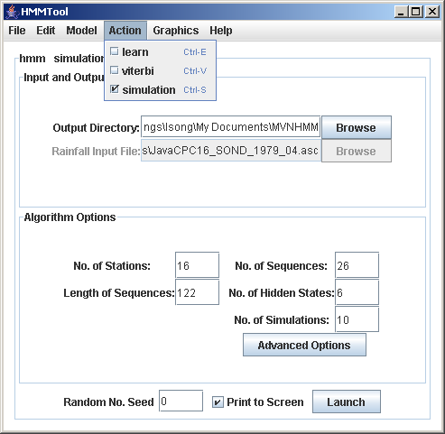
Once the model parameters have been estimated, the model can be used to make a set of rainfall simulations, using the simulate action from the Action Menu. When simulate is selected, an additional option appears on the Main Frame to specify the number of simulations. If the dataset has 30 sequences of 90 days, 2 simulations would produce 2 sets of 30 sequences of 90 days, with the second set below the first set. No advanced options need to be changed. Once simulate has been selected, simply click Launch on the main frame.The stochastic simulations are written to a *.out file in the output directory, with the filename including the word 'simulation' .The simulations can be analyzed off-line to test the model performance in terms of key statistics, such as dry-spell run lengths, for example.The most appropriate number of hidden states (k) is a subjective choice based on the goal of the analysis. It can be guided by the BIC (Bayes Information Criterion, a penalized likelihood measure) values obtained with different choices of k, found in the 'learn'.out files. A graph of the BIC vs. k (for k = 2 .. 15, say) will generally increase with k to a certain point, before reaching a maximum or a plateau. The smallest k for which the BIC no longer increases appreciably makes a reasonable choice, although examination of the states themselves in terms of composites of atmospheric winds etc can provide further guidance.5. Introducing Predictors
The NHMM and NMIXTURE model types require an additional predictor input file on the Main Frame, that specifies the timeseries of a set of predictors. For the learn and Viterbi actions, this file needs to have the same number of rows (number of sequences x sequence-length) as the rainfall data. Each whitespace-delimited column of the file should contain a separate predictor, with the number of columns matching the number of predictors specified in the main panel.For the simulation action, the number of rows in the predictor input file must match the desired length of the simulations.The output files from the Viterbi and simulation actions with predictors have the same form as for models without predictors. However, note that the learn action with predictors produces an output file of a sightly different form, because there is no simple transition matrix in this case. A transition matrix can be reconstructed from the Viterbi sequence.