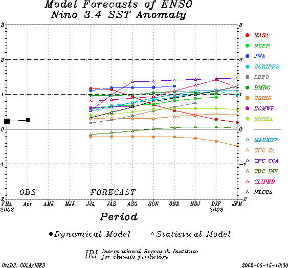
16 May, 2002

Interpreting the model forecasts...

The following graph and table show forecasts made by both dynamical and statistical models for sea surface temperatures in the Nino 3.4 region for eight overlapping 3-month periods.  It should be noted that the expected skills of the models, based on historical performance, are not equal to one another. The skills also generally decrease as the lead time increases. Thirdly, forecasts made at some times of the year generally have higher skill than forecasts made at other times of the year- for example, there is generally more skill for forecasts made between June and October than those made between January and April. Differences among the forecasts shown on the graph and in the table reflect both differences in model design, and actual uncertainty in the forecast of the possible future SST scenario.

The set of dynamical and statistical model forecasts issued during late April and early May shows a range of possible sea surface temperature conditions for the coming 3 to 8 months (June-July-August through January-February-March 2003). More models are indicating a warming tendency than a neutral outlook, and none are calling for cold conditions. A sizeable proportion of models forecast significant warming (e.g., warming to 0.6 degrees C or more above average in the Nino 3.4 region for the July-August-September seasonal average). A noticeable fraction are also forecasting ENSO conditions in the upper half of the neutral category-between 0.0 and 0.5 degrees C above normal. The warmest forecast for the July-August-September period comes from the dynamical model of the Japanese Meteorological Agency (1.2 degrees C above normal), and the coldest one is from the Australian CSIRO/COCA dynamical model, calling for SST anomalies of -0.2 degrees C. For later in the year, such as September-October-November or later, eight of the fourteen models that forecast to that long a lead time suggest El Nino development: the NASA/NSIPP, NCEP coupled, JMA, Scripps, BMRC, CPC Markov, CPC-CCA, Colorado State CLIPER, and the UBC nonlinear CCA.

FORECAST SST ANOMALIES (deg C) IN NINO 3.4 REGION

Some notes about the formulation of the entries in the table above:

=>Only models producing forecasts on a monthly basis are included. This means that some models whose forecasts appear in the Experimental Long-Lead Forecast Bulletin (produced by COLA) do not appear in the table (e.g. the COLA forecasts).

=>The SST anomaly forecasts are for the 3-month periods shown, and are for the Nino 3.4 region (120-170W, 5N-5S). Often, the anomalies are provided directly in a graph or a table by the respective forecasting centers for the Nino 3.4 region. In some cases, however, they are given for 1-month periods, for 3-month periods that skip some of the periods in the above table, and/or only for a region (or regions) other than Nino 3.4. In these cases, the following means are used to obtain the needed anomalies for the table:

o temporal averaging,

o linear temporal interpolation,

o visual averaging of values on a contoured map, and

o regional SST anomaly adjustment using the climatological variances of one region versus that of another.

As an example of the last case, suppose only the Nino 3 anomaly is provided. The Nino 3.4 anomaly is then obtained by decreasing the Nino 3 anomaly by the factor defined by the ratio of the year-to-year variance of Nino 3.4 to the year-to-year variance of Nino 3 SST, for the 3-month season in question.

The anomalies shown are those with respect to the base period used to define the normals, which vary among the groups producing model forecasts. They have not been adjusted to anomalies with respect to a common base period. Discrepancies among the climatological SST resulting from differing base periods may be as high as a quarter of a degree C in the worst cases. Forecasters are encouraged to use the standard 1971-2000 period as the base period, or a period not very different from it.