Use of a regularized EM algorithm to fill very gappy Malaria data
Previous gap-filling techniques were not very satisfying in order to produce a synthetized analysis of the available dataset, whether because the dataset had to be split, or the choice of some time series to be discarded didn't seem fair, or because more than half of them had to be discarded. Here, a regularized EM algorithm is applied, discarding just a few time series, and filling all the remaining gaps. This page shows the results of such analysis with the default values provided.
The covariance matrix
The Singluar Value Decomposition (SVD), when applied to the whole very gappy dataset, was discarding an important number of time series which had a number of data points significantly higher than other time series that were not discarded. That process didn't seem fair and called for a modification in the analysis. It appears that the SVD is compressing the gappy covariance matrix with a criterium that relied on the number of time series a given time series would have covariance with, disregarding the richness of the covariance information, since one common point alone between two time series is enough to get a covariance. Of course, that criterium gets rid of the very poor time series, but, because of the configuration of this dataset with two obvious subsets, very poor time-series would be preserved because they have a covariance with more time series than richer time series stuck in a longer subset but with less time series.
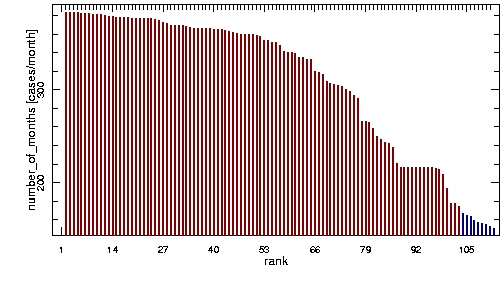
A simple solution to that issue is to get rid of the too poor time series before the analysis until that side effect is eliminated. To do so, 39% of the poorest time series had to be discarded which is not very satisfying as Figure 1 shows.


Figure 1 - After discarding 39% of the poorest districts: ranked by number of points in time series, blue districts are the ones discarded by SVD.
There had to be a way to change the way the covariance matrix was compressed, or even estimate a covariance matrix from the available information. A regularized Expectation-Maximization (EM) algorithm estimates the covariance matrix iteratively, in this case discarding only nine districts (two of them being empty of data points). In an iteration of the EM algorithm, given estimates of the mean and of the covariance matrix are revised in three steps. First, for each record with missing values, the regression parameters of the variables with missing values on the variables with available values are computed from the estimates of the mean and of the covariance matrix. Second, the missing values in a record X are filled in with their conditional expectation values given the available values and the estimates of the mean and of the covariance matrix, the conditional expectation values being the product of the available values and the estimated regression coefficients. Third, the mean and the covariance matrix are re-estimated, the mean as the sample mean of the completed dataset and the covariance matrix as the sum of the sample covariance matrix of the completed dataset and an estimate of the conditional covariance matrix of the imputation error.
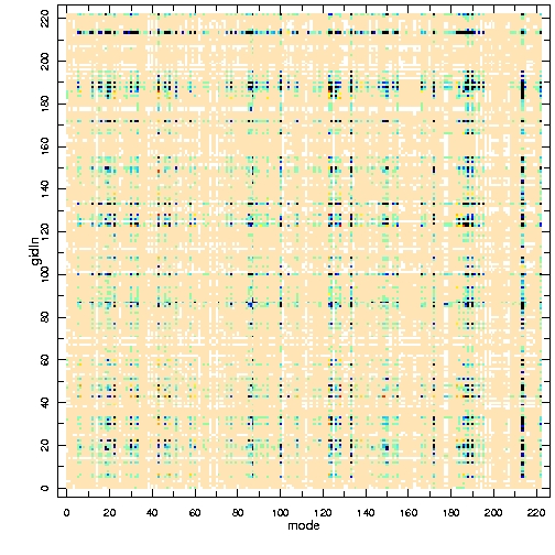
As default initial condition for the imputation algorithm, the mean of the data is computed from the available values, mean values are filled in for missing values, and a covariance matrix is estimated as the sample covariance matrix of the completed dataset with mean values substituted for missing values. Figure 2 shows the original gappy covariance matrix, the estimated one and their difference.


Figure 2 - From left to right, the gappy covariance matrix of the original dataset; the one estimated by EM; the difference between both.
The reconstruction
In the regularized EM algorithm, the parameters of the regression models are estimated by a regularized regression method. By default, the parameters of the regression models are estimated by a multiple ridge regression for each record with missing values, with one regularization parameter per record with missing values. The regularization parameters for the ridge regressions are selected as the minimizers of the generalized cross-validation (GCV) function.
The multiple ridge regression computes the regularized estimate of the coefficient matrix in the multivariate multiple regression model Y = X*B + noise(S), via an eigendecomposition of the covariance matrix.
GCV offers a way to estimate appropriate values of the ridge regularization parameter. The GCV function to be minimized has the form of the ratio of the squared residual norm, by a squared effective number of degrees of freedom (see details in reference below). Both numerator and denominator increase with increasing regularization, the GCV function attempts to find a good trade-off between the two.
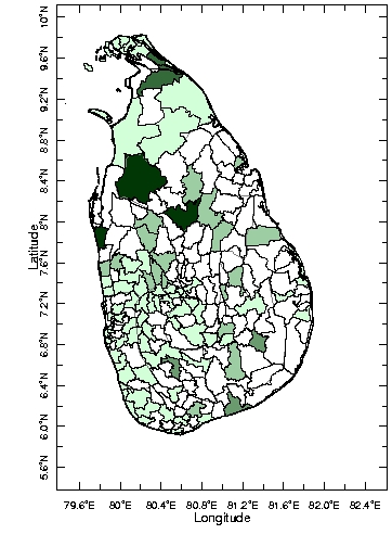
Figure 3 shows an estimated standard error of the imputed values provided by the analysis.


Figure 3 - Estimated error of the imputed values by EM; it is set to 0 where there were actual data.
Further description about the EM algorithm is available here.
The cluster analysis
A new cluster analysis is performed on this non-gappy dataset. A clickable Figure 4 shows the results.


Figure 4 - Cluster analysis of the EM gap-filled Sri Lanka malaria data. Click on the map to have access the cluster overview
Overall, the result of this analysis is coherent with all the previous ones. The first cluster is formed by those three districts which explain the biggest fraction of the variance. The third cluster is composed by the two northern districts that we know experience this 1995-2003 event. Cluster 2 and 4 gathers those districts that each previous analysis was clustering in different ways. The fourth cluster is composed of three districts having a pike in 1997-1998 whereas the second cluster is composed of thirty four districts with relatively low variability. The fifth cluster is more or less the same cluster with the remaining districts.